AVERAGEIFS function

AVERAGEIFS function



This article describes the formula syntax and usage of the AVERAGEIFS function in Microsoft Excel.



Description Returns the average (arithmetic mean) of all cells that meet multiple criteria.



Syntax AVERAGEIFS(average_range, criteria_range1, criteria1, [criteria_range2, criteria2], ...) The AVERAGEIFS function syntax has the following arguments:

• Average_range Required. One or more cells to average, including numbers or names, arrays, or references that contain numbers.
• Criteria_range1, criteria_range2, ... Criteria_range1 is required, subsequent criteria_ranges are optional. 1 to 127 ranges in which to evaluate the associated criteria.
• Criteria1, criteria2, ... Criteria1 is required, subsequent criteria are optional. 1 to 127 criteria in the form of a number, expression, cell reference, or text that define which cells will be averaged. For example, criteria can be expressed as "31", "31", "> 31", "apples", or B4.

Remarks

• If average_range is a blank or text value, AVERAGEIFS returns the #DIV0! error value.
• If a cell in a criteria range is empty, AVERAGEIFS treats it as a 0 value.
• Cells in range that contain TRUE evaluate as 1; cells in range that contain FALSE evaluate as 0 (zero).
• Each cell in average_range is used in the average calculation only if all of the corresponding criteria specified are true for that cell.
• Unlike the range and criteria arguments in the AVERAGEIF function, in AVERAGEIFS each criteria_range must be the same size and shape as sum_range.
• If cells in average_range cannot be translated into numbers, AVERAGEIFS returns the #DIV0! error value.
• If there are no cells that meet all the criteria, AVERAGEIFS returns the #DIV/0! error value.
• You can use the wildcard characters, question mark (?) and asterisk (*), in criteria. A question mark matches any single character; an asterisk matches any sequence of characters. If you want to find an actual question mark or asterisk, type a tilde (~) before the character.

Note: The AVERAGEIFS function measures central tendency, which is the location of the center of a group of numbers in a statistical distribution. The three most common measures of central tendency are:

• Average which is the arithmetic mean, and is calculated by adding a group of numbers and then dividing by the count of those numbers. For example, the average of 2, 3, 3, 5, 7, and 10 is 30 divided by 6, which is 5.
  
  The mathematical Mean is the same as the Average function. The formula is
  
  
  
  
  
  
  
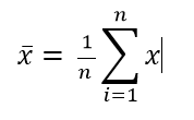
  Where :
  
  x?? - Mean or Average of the numbers.
  
  n - is the sample size of Number of elements.
  
  x - The value of each element or number in the data set.
  
  
  
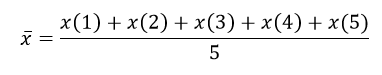
  To find the mean(average) of 5 numbers this would expand as below:
  
  
  
  
• Median which is the middle number of a group of numbers; that is, half the numbers have values that are greater than the median, and half the numbers have values that are less than the median. For example, the median of 2, 3, 3, 5, 7, and 10 is 4.
• Mode which is the most frequently occurring number in a group of numbers. For example, the mode of 2, 3, 3, 5, 7, and 10 is 3.

For a symmetrical distribution of a group of numbers, these three measures of central tendency are all the same. For a skewed distribution of a group of numbers, they can be different. Examples Copy the example data in the following table, and paste it in cell A1 of a new Excel worksheet. For formulas to show results, select them, press F2, and then press Enter. If you need to, you can adjust the column widths to see all the data. Example 2